Abstract
Quillwave reconstructs a full 256×256 ripple field from 64 point sensors. Ripple fields are procedurally generated sums of interfering circular waves: cheap to synthesise, but hard to interpolate, because the wave fronts between sensors are lost by smooth interpolation. Quillwave encodes the sensor readings into a 128-dimensional latent field code and decodes it with a coordinate-based field decoder. On RippleBench-Synthetic, a benchmark of 500 synthetic test fields generated for this work, Quillwave reaches 29.46 dB PSNR and 0.887 SSIM, 5.41 dB above radial-basis interpolation (the best baseline), which is a 71.2% lower mean squared error. It is also 1.36× faster than radial-basis interpolation at inference. All results are on synthetic fields only.
Video
Read the transcript (the video has on-screen captions and no speech) · Download the video (MP4)
Method
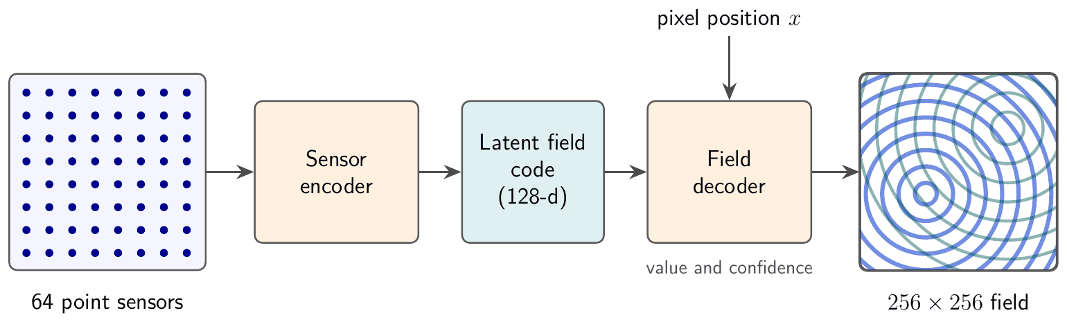
The input is 64 point sensors on a regular 8×8 grid. A sensor encoder maps the readings to a 128-dimensional latent field code. A coordinate-based field decoder then predicts the field value and a confidence at every pixel, so the output resolution is not tied to the training resolution (all results here use the benchmark resolution). Quillwave-Lite is the ablation without the latent code: its decoder is conditioned on the raw readings. The full model has 1.2M parameters and was trained on 2000 synthetic fields for 200 epochs.
Results
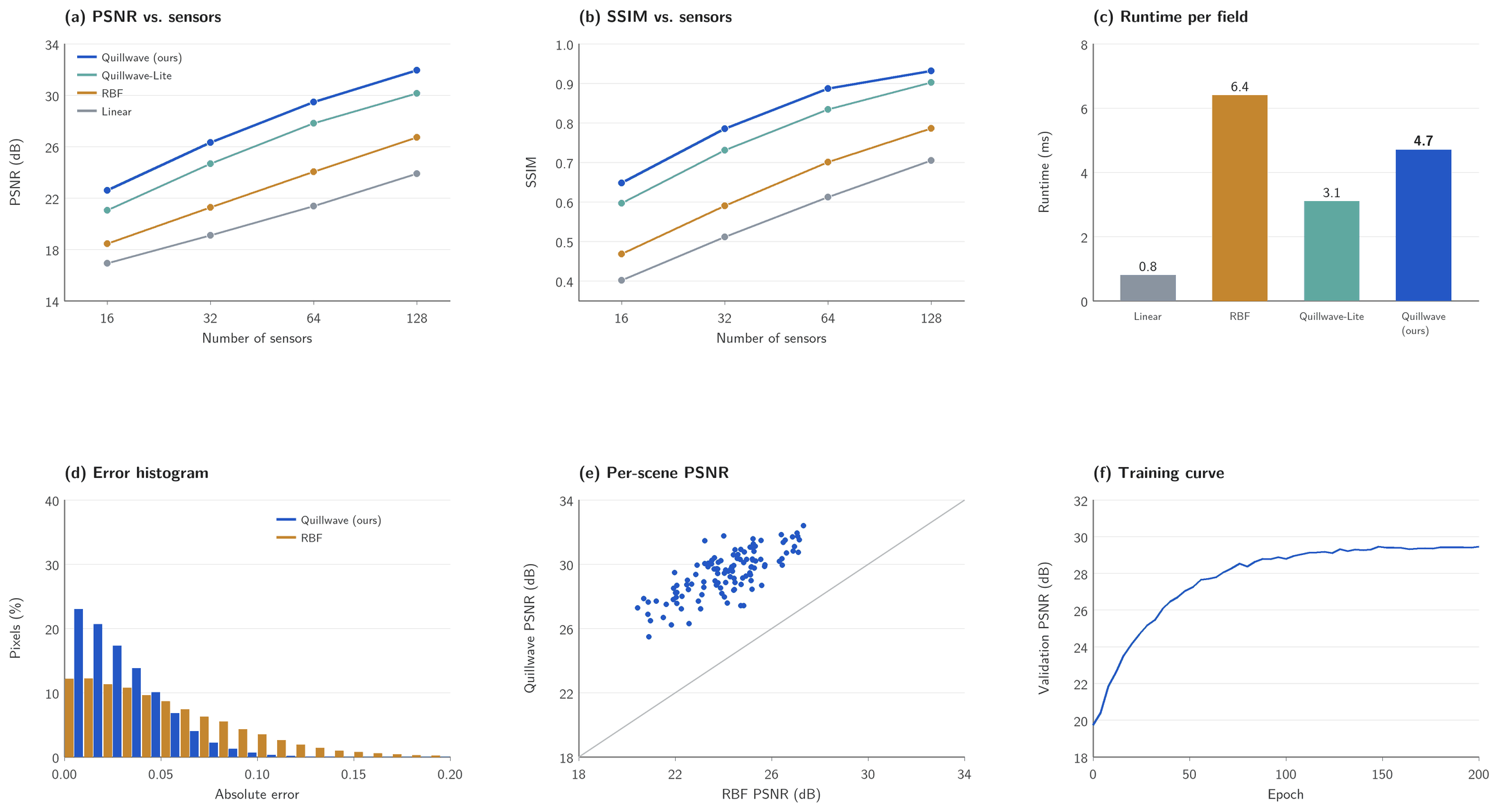
Quillwave reaches 29.46 dB PSNR and 0.887 SSIM on RippleBench-Synthetic with 64 sensors. That is 5.41 dB above radial-basis interpolation, the best baseline, a 71.2% reduction in mean squared error, and it runs 1.36× faster than that baseline (4.7 ms against 6.4 ms), though slower than linear interpolation (0.8 ms). Quillwave-Lite reaches 27.82 dB, so the latent field code accounts for part of the gain. Quillwave is the best method at every sensor count from 16 to 128.
Table 1. Reconstruction quality on RippleBench-Synthetic (64 sensors, 256×256 fields, mean over 5 training runs). Higher PSNR/SSIM is better; lower runtime is better.
| Method | PSNR (dB) | SSIM | Runtime (ms) |
|---|---|---|---|
| Linear interpolation | 21.37 | 0.612 | 0.8 |
| Radial-basis interpolation | 24.05 | 0.701 | 6.4 |
| Quillwave-Lite (ablation) | 27.82 | 0.834 | 3.1 |
| Quillwave (ours) | 29.46 | 0.887 | 4.7 |
Table 2. PSNR (dB) on RippleBench-Synthetic as the number of sensors changes (256×256 fields).
| Method | 16 sensors | 32 sensors | 64 sensors | 128 sensors |
|---|---|---|---|---|
| Linear interpolation | 16.92 | 19.10 | 21.37 | 23.88 |
| Radial-basis interpolation | 18.44 | 21.26 | 24.05 | 26.71 |
| Quillwave-Lite (ablation) | 21.03 | 24.67 | 27.82 | 30.15 |
| Quillwave (ours) | 22.58 | 26.31 | 29.46 | 31.94 |
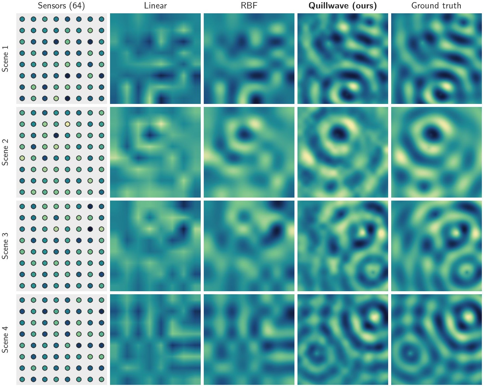
Comparison Clips
Limitations
- Baselines are not compute-matched. Quillwave is trained for 3.5 GPU-hours, while the interpolation baselines need no training at all.
- Synthetic fields only. Every result is on RippleBench-Synthetic; no real sensor data was used, and behaviour on real measurements is unknown.
- Confidence is not calibration. The per-pixel confidence map that Quillwave outputs has not been checked against observed error rates, so it should not be read as a calibrated probability.
BibTeX
@inproceedings{placeholder2026quillwave,
  title     = {Quillwave: Sparse-Sensor Reconstruction of Synthetic Ripple Fields},
  author    = {Ada Placeholder and Ben Example and Cleo Sample},
  booktitle = {Proc. FCSV 2026 (Fictional Conference on Synthetic Vision)},
  year      = {2026},
  url       = {https://quillwave.example.org/},
  note      = {Fictional entry for testing}
}